Technical Note

Radioelement Anomaly Detection

The GammaSpec "Anomaly Detection" tool (Enhancements|Anomaly Detection) is capable of detecting radioelement anomalies from both line and grid data. The method detects 3 types of anomalies: 

• Spectral anomalies are those areas on the map where the 3-component radioelement signature (K, U and Th concentrations) are rare. They do not necessarily have anomalous amplitudes. Spectral anomalies are a type of vector anomaly.
• Potassic anomalies are a special type of spectral anomaly. They show areas where there is potential enrichment of K relative to Th. 
• Point anomalies are the classical geophysical anomalies with anomalous amplitudes above a local background. 

The anomaly types are described in more detail below.

Spectral Anomalies

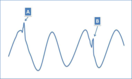
Consider the schematic shown in the schematic below, which represents a hypothetical dataset. The value at anomaly “A” occurs only once in the entire dataset – its value is rare. I call this a “spectral” anomaly. In the case of 3-component radioelement data, spectral anomalies are those areas of the map (or profiles) where the 3-component radioelement signatures (K, U and Th concentrations) are rare. They do not necessarily have anomalous amplitudes – rather, it is the relative concentrations of K, U and Th (i.e. the ratios between the radioelement concentrations) that is anomalous. Spectral anomalies are thus 3-component vector anomalies.

This is the main difference between spectral and point anomalies – spectral anomalies are vector anomalies whereas point anomalies are scalar. Spectral anomalies can also be viewed from a principal component analysis perspective. The lowest-order principal component of a multivariate dataset is that component that accommodates most of the variance in the dataset. Higher-order components accommodate successively less of the variance in the dataset. Spectral anomalies can be thought of as those parts of the (K, U, Th) vector space that have the least-common signature. They are those areas of the map that are most different from the mean.

Spectral anomalies may, or may not, be important from a mapping or mineral/petroleum exploration perspective. But because they have unusual signatures, they need to be identified and assessed. 

Potassic Anomalies

Potassic anomalies are a special class of spectral anomalies. They are spectral anomalies that display high K values relative to Th. There is a considerable body of literature suggesting that these anomalies may be indicators of potassic alteration. 

Point Anomalies

Point anomalies are the classical geophysical anomalies comprising anomalous amplitude above a local background. With reference to schematic above, the value at point “B” occurs at several places in the dataset – so the actual data value at B is not rare. But it is anomalous with respect to the local background. We call these “point” anomalies. 

Point anomalies are found by looking at the correlation between a theoretical anomaly and the actual data at every point on a grid or along a line profile. Anomalies are found where the correlation (or “goodness-of-fit”) between the actual and theoretical exceeds a nominal threshold value. The centre of the anomaly is at the point of maximum correlation. 

Point anomalies are contextual anomalies – they are anomalous within a local context, and have measurable amplitude. They are also scalar quantities – just one of K, U or Th can give rise to a point anomaly. 

Program Control

Spectral anomalies can also be considered as contextual in the sense that the 3-component data are assessed as to how different they are from the prevailing background values. The background values can be either the mean values for the whole survey, or a local mean in the vicinity of the data being assessed. GammaSpec is capable of producing spectral and potassic anomalies from grid data using either the whole survey to estimate the mean values (referred to as a “regional” background), or a more local area in the vicinity of the data being assessed (referred to as a “local” background) by using "tiles". The grid is sub-divided into overlapping tiles for processing. For line data, the use of a regional background only is supported. 

The spectral and potassic anomalies derived using a regional background are likely to be more useful for lithological mapping purposes, as the criteria used for their selection are consistent for the entire survey. They are also more likely to show the main deviations from the mean. On the other hand, the spectral and potassic anomalies derived using a local background are likely to be more useful for the detection of more subtle anomalies, and perhaps also the direct detection of altered or mineralized zones. There is a tendency for anomalies detected using a local background to be more evenly spread across a survey area. Depending on the geology, it is possible for the majority of anomalies detected using a regional background to be concentrated in specific areas. 

For the detection of point anomalies, the user specifies the parameters that define a theoretical anomaly that is used as a matched filter. The number of points in these anomalies should be carefully chosen through trial and error. The filter coefficients are listed in the output log file. As a rule of thumb, choose the number of coefficients in the filter such that the outer coefficients fall to just below 10% of the value in the centre of the filter. 

Program Output

GammaSpec outputs anomalies to ESRI shape files. The anomaly attributes for spectral and potassic anomalies are the same, and are listed in Table 1. The anomaly attributes for point anomalies are slightly different, and are listed in Table 2. These attributes can be used within a GIS to selectively display anomalies to assist in their interpretation. Any additional anomaly attributes present in the shape files are program control parameters for internal use by Minty Geophysics. 

Point anomalies are often used in uranium exploration for the direct detection of mineralization. The two shape file attributes that are most useful for the assessment of point anomalies are the anomaly amplitude (AnomalyAmpl) and the goodness-of-fit (AnomalyFit). Point anomalies are found by convolving a theoretical anomaly (due to a vertical prism) with the radioelement profiles or grids. Anomalies are detected where the goodness-of-fit exceeds a certain threshold. However, small-amplitude anomalies are more affected by noise than large-amplitude anomalies, and it is unreasonable to expect a high goodness-of-fit for small-amplitude anomalies. So there is a connection between the goodness-of-fit and anomaly amplitudes. 

The anomaly amplitudes in the shape files are not in the conventional radioelement concentration units (% for K, and ppm for eU and eTh). In order to facilitate comparison between anomaly amplitudes for mixed anomaly types (eg. U+Th), they are expressed in units of the average crustal concentrations of the radioelements (2 % K, 2.5 ppm eU and 9 ppm eTh). So, for a pure uranium anomaly with amplitude 2.0, the actual peak of the anomaly above local background is 5 ppm eU. 

Table 1:  Spectral and potassic anomaly attributes.

Table 2:  Point anomaly attributes.