
Technical Note
Portable Gamma-Ray Spectrometry
There are a few fundamental differences between airborne and portable gamma-ray spectrometry due to the following:
- Airborne measurements are made from a moving platform, and to achieve a reasonable spatial resolution the measurement times are small – typically 0.5 s or 1 s. This means that airborne spectra are noisy. Portable measurements typically use large integration times (e.g. 300-600 s) to improve the precision of the radioelement estimates. NASVD-type analysis to reduce noise are thus not generally applied to portable spectrometer measurements. However, if sufficient spectra are available, then NASVD analysis will result in greater precision.
- Background radiation, as a proportion of the total radiation, is far greater for airborne measurements than for portable spectrometer measurements on the ground. The radon background alone, for example, can be many times the radiation due to uranium from the ground for airborne surveys. The background correction for portable spectrometry is therefore much simpler – typically, an estimate of total background is made for the survey area and this is subtracted from all measurements in the survey.
- Airborne measurements are severely affected by deviations in the height of the detector from the nominal survey height, and must be corrected for these deviations. A height correction is not necessary for portable measurements as spectra are recorded at ground level.
- The window sensitivities for airborne detectors are estimated from flights over a calibration range, as this is the only way to measure the detector response to semi-infinite sources. However, because portable spectrometers can be placed directly onto calibration pads, reasonably accurate estimates of their window sensitivities can be obtained from these measurements by applying a correction for the finite size of the pads.
Both airborne and portable spectrometry assume a semi-infinite plane surface (a broad source) as the most common source type encountered during surveying, and the spectrometers are calibrated accordingly. This assumption is more reasonable for airborne spectrometry than for portable spectrometry. Deviations from a flat, plane surface in the vicinity of the measurement site is common for portable spectrometry, and these introduce bias into the final radioelement estimates. So, while radioelement estimates form airborne measurements are not very precise, they are reasonably accurate, as the assumption of plane sources is more easily met. On the other hand, radioelement estimates from portable measurements may be very precise (due to large sample times), but are not necessarily accurate if the earth's surface in the vicinity of the measurement does not approximate a plane surface.
Instrumentation and Measurement
Portable spectrometers will have at least 350 cm3 of NaI Detectors, although smaller hand-held instruments using BGO detectors are now available. The spectrometers are otherwise similar to airborne instruments, recording at least 256-channel spectra with automatic energy stabilisation. Calibration constants can be stored inside the instruments, giving real-time output in concentrations of the radioelements. However, as with airborne instruments, slow drift of the base level means that it is advisable to post-process the recorded spectra to get more accurate results.
Portable spectrometer data can be acquired two ways. Measurement at fixed locations on the ground (static mode) has the advantage of using long sample integration times to improve measurement precision. Recordings can also be made in a continuous streaming mode (dynamic mode), similar to airborne surveys, as the operator walks along designated lines, or in vehicle-borne surveys. However, measurements along a traverse are only comparable if the source-detector geometry is the same for each measurement. To minimise geometry effects, the spectrometer is best placed on the ground for static measurements (Figure 1).
Figure 1. Portable spectrometer measurements
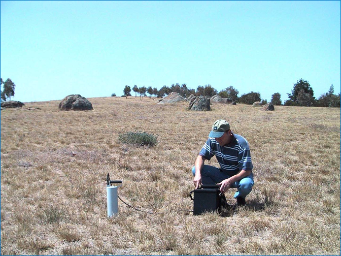
As with airborne surveys, the height of the detector affects the area being sampled. For example, a detector placed on the ground will sample a volume of rock/soil about 25 cm thick and 2 m in diameter. For measurements above the ground, the source material being sampled could be several meters or even tens of meters in diameter.
Calibration
The calibration of portable spectrometers entails the estimation of background radiation, stripping ratios and window sensitivities. The background radiation is a combination of the instrument background (the internal radioactivity of the spectrometer), cosmic background and atmospheric radon background. The IAEA (IAEA, 2003) recommends measuring the total background radiation over a lake or river from a small boat (preferably fibreglass), and at least 200m from the shore. This should be done as close as possible to the survey area, and at the same time as the survey.
Stripping ratios and sensitivities are derived from measurements over the same concrete calibration pads used for airborne spectrometer calibrations (Figure 2).
Figure 2. Calibrating a portable spectrometer on calibration pads
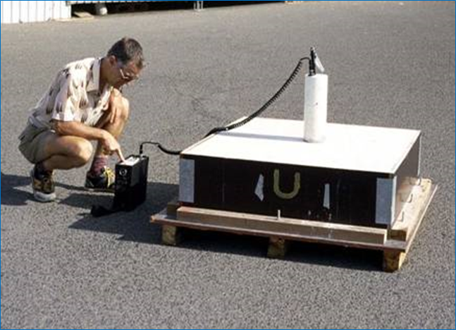
Each calibration pad has a known concentration of the radioelements. Three of the pads are preferentially doped with one of K, U and Th. And the fourth pad (the "background" pad) has concentrations similar to the impurities in each of the other pads. Measurements are taken on each of the pads, and the K, U and Th pad measurements are corrected for the ambient background (all sources other than the calibration pad) by subtracting the measurements obtained over the background pad. These background-corrected counts are are linearly related to the background-corrected concentrations in the respective K, U and Th pads (K, U and Th pad concentrations minus the concentrations in the background pad) as follows:
ni = siKcK + siUcU + siThcUTh
where ni = count rate in the i-th energy window (K, U or Th);
sij = sensitivity of the i-th energy window to the j-th radioelement (cps per unit concentration);
cj = concentration of the j-th element (% K, ppm U and ppm Th).
In matrix notation this can be written as
N = SC,
with the solution
S = NC-1
The stripping ratios are derived from the sensitivity matrix as follows:
α = s2Th/s3Th β = s1Th/s3Th γ = s1U/s2U
a = s3U/s2U b = s3K/s1K g= s2K/s1K
The K, U and Th window sensitivities are the diagonal elements of the sensitivity matrix. These must be adjusted (scaled upward) to correct the sensitivities for the finite size (and densities) of the calibration pads, and the height of the detector crystal (inside its housing) above the surface of the pads. Typical correction factors are 1.14, 1.16 and 1.17 for the K, U and Th pads respectively.
The GammaSpec “Portable Pad Calibration” tool (Portable|Portable Pad Calibration) calculates the window backgrounds from an over-water spectrum, and the stripping ratios and sensitivities from pad calibration data.
Processing
The processing sequence for portable gamma-ray spectrometry is as follows:
- Energy calibration of the gamma-ray spectra
- Live-time correction and windowing
- Removal of background radiation
- Stripping (channel interaction correction)
- Sensitivity correction (reduction to elemental concentrations)
The energy calibration, live-time correction and windowing are the same as for the processing of airborne spectra. Portable spectrometers don’t usually report a deadtime/livetime. Rather, the sampling interval is automatically extended such that the reported sampling time is already corrected for dead time. The live-time correction is then simply the conversion of the window counts to counts per second by dividing by the sample time in seconds.
The measured over-water backgrounds are subtracted from the window count rates. The background-corrected window count rates are then stripped. Usually, the stripping ratios b and g are assumed 0. In this case, if K, U and Th are the background-corrected window count rates then the stripping equations become
Thcorr = (Th – aU) / (1 – aα)
Ucorr = (U – αTh) / (1 – aα)
Kcorr = K – βThcorr – γUcorr
where Kcorr, Ucorr and Thcorr are the stripped window count rates.
Finally, the stripped window count rates are converted to concentrations by dividing them by the appropriate sensitivity coefficient
C = N/S
where C are the concentrations, N are the background-corrected and stripped window count rates, and S are the sensitivities. The concentrations are the elemental concentrations (% K, ppm U and ppmTh) which would give rise to the observed count rates if the radioelements were evenly distributed through an infinite slab source.
The GammaSpec “Portable Processing” tool (Portable|Portable Processing) processes raw gamma-ray spectra to final concentrations of the radioelements.
References
IAEA, 2003. Guidelines for radioelement mapping using gamma-ray spectrometry data. IAEA-TECDOC-1363, International Atomic Energy Agency, Vienna.